Precomputed Radiance Transfer
Keywords:
tutorial,
X3D,
Avalon,
rendering,
PRT
Author(s): Tobias Alexander Franke
Date: 2008-06-23
Summary: This tutorial teaches you how to use precomputed radiance transfer.
Introduction
Precomputed Radiance Transfer (PRT) is a technique to lift lighting calculations to frequency space. The major advantage to this method is a massive rendering speed improvement for global illumination. Consider the rendering equation being broken down to an double integral product, where L_o is the total amount of radiance along Omega_r, L_e is emitted light, L_i is inward light from a light source in the hemisphere and f is the BRDF:
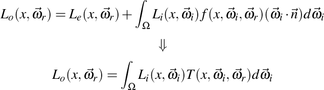
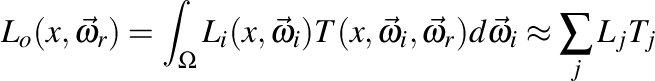
PRT shortens the general rendering equation to an integration of incident lighting and a so called transfer function T, which includes all other terms inside the integral. Assuming that the rendered object is rigid, the transfer function stays fixed, meaning that computationally intenisve parts can be precomputed. From Fourier analysis we know that integration in position space can be turned into a dot product in frequency space. So by transferring both terms - the incident lighting and the transfer function - to frequency space with a suitable basis, the integral can be approximated in real time:
This trick has major runtime implications: regardless of the transfer function complexity, the result can be compressed and uploaded to shader as a vector of coefficients, where it is dotted with a lighting vector to calculate the result of the equation. Depending on the transfer function complexity, different basis functions yield different results that are more or less suited to represent it in a compressed way. For instance, the popular spherical harmonic basis used in most PRT simulations is very suitable for low-frequency reflections, like diffuse shaded surfaces, but almost useless for highly reflective materials. Whatever the basis is going to be at the end is therefore a matter of what kind of transfer one wants to simulate.
For the uninitiated, a very good overview and tutorial - Spherical Harmonics: The Gritty Details by Robin Green - should serve as a more clarifying introduction. In addition, this X3D tutorial is based on the Web3D 2008 paper by Tobias Alexander Franke and Yvonne Alexandra Jung Precomputed Radiance Transfer for X3D based Mixed Reality Applications.
Practical issues
Instant Reality is a rendering framework and thus does not provide a rendering application to compute the coefficients for your object. However, writing such an application is not very complicated, but does require some planning ahead. In this section, we'll take a closer look at what's really needed.
The first thing to be done is to precompute the coefficients needed for the transfer function. The transfer function is defined for each surface point and needs to be sampled, converted and saved with the object you want to display. Let's start out with an easy example. Imagine the transfer function at each vertex of an object is defined as:
This transfer function simply includes the Lambert term multiplied with a visibility function, which tests if a surface point x is occluded by some other geometry in direction Omega_i. Implementation wise, at each vertex the renderer takes a certain amount of samples, say 1000, with a raytracer, testing the hemisphere for occlusion with the object's own geometry, and multiplies the result (which is either 0 for occlusion or 1 for no occlusion) with the Lambert term and the basis function value for the same Omega_i. Dividing this sum by 1000 yields the coefficient for the base function. A simple and straightforward implementation can be found in Spherical Harmonics: The Gritty Details by Robin Green.
The coefficients, for low frequency reflections, come as groups called bands, and the number of coefficients is the number of bands squared, so 3 bands yield 9 coefficients. These coefficients later need to be uploaded to the graphics card, where they are combined with another vector representing the incidient lighting function. So the remaining question to solve is: How do we upload these coefficients to the GPU? There are a lot of different ways to do this. For instance, one could save the coefficients in texture maps that are uploaded together with the object. The probably easiest and most straightforward way is to use the available vertex attributes. Since color, normal and certain texture coordinate attributes are not needed after all the material or transfer info has been encoded in the coefficients, these empty slots can be filled up - a good way is thus to save the coefficients with the attributes directly. The Instant Player will load these models just like any other, and the shader will have access imidiatly to these coefficient values.
As an example, let's imagine that we have calculated 3 bands, i.e. 9 coefficients, for each transfer function. There are four color channels per vertex (in case of SFColorRGBA); three values for the vertex normal (x, y, and z), and two texture coordinate fields for textures. We can replace the values in these now unused slots with coefficient values. Later on, those values will turn up on our shader, were we do not use them as values for color, normal and texture coordinate, but again as coefficients. If you need the color values though, you might also move the coefficient values to all the texture coordinate attributes. Again, this is largely a design question of how and what your final object will use to display the surface material.
The following X3D example shows a sample configuration for 4 bands, i.e. 16 coefficients, encoded per vertex via texture coordinate fields. Here, each texture coordinate field is saving 4 values per vertex, so four TextureCoordinate4D fields are needed to save all 16 coefficients. Attached to this tutorial is a sample model with calculated PRT data for 4 bands saved in the same way.
Code: X3D encoding PRT data in texture coordinates.
<Shape>
	<Appearance>
		...
	</Appearance>

	<IndexedFaceSet coordIndex=' ... '>

		<Coordinate point=' ... ' />
		<Normal vector=' ... ' />
		<Color color=' ... ' />

		<!-- PRT DATA GOES HERE -->
		<MultiTextureCoordinate>
			<TextureCoordinate4D point=' ... ' />
			<TextureCoordinate4D point=' ... ' />
			<TextureCoordinate4D point=' ... ' />
			<TextureCoordinate4D point=' ... ' />
		</MultiTextureCoordinate>

	</IndexedFaceSet>
</Shape>
X3D and PRT
So far there is no support for PRT in X3D available. However, the Instant Reality framework does provide two minimal tools needed to use PRT in your application. Since all coefficients are now saved up with the model, the remaining question is how to to calculate the coefficient vector for the incident light.
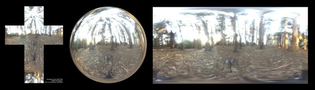
The Instant Reality framework provides a node called SphericalHarmonicsGenerator, which is designed specifically for this task. A spherical image - be it a latitude-longtitude-, sphere- or cubemap - is converted to a vector of coefficients at runtime.
Code: Converting a spherical image to coefficients.
<Appearance>
	<ComposedShader DEF='shShader'>
		<field accessType='inputOutput' name='coefficients' type='MFVec3f' value='
			0 0 0
			0 0 0 0 0 0 0 0 0
			0 0 0 0 0 0 0 0 0 0 0 0 0 0 0
			0 0 0 0 0 0 0 0 0 0 0 0 0 0 0 0 0 0 0 0 0'/>
		<ShaderPart type='vertex' url='"prt_vp.glsl"'/>
		<ShaderPart type='fragment' url='"prt_fp.glsl"'/>
	</ComposedShader>
	...

	<SphericalHarmonicsGenerator DEF='shGenerator' bands='4' mapMode='latLong'>
		<ImageTexture DEF='sphericalImage' url='"latlong.hdr"'/>
	</SphericalHarmonicsGenerator>
</Appearance>
...

<ROUTE fromNode='shGenerator' fromField='coefficients_changed' toNode='shShader' toField='coefficients'/>
As we can see from the code, the SphericalHarmonicsGenerator has an input texture called irradianceMap (which should be a high dynamic range image), and the type of texture is set with mapMode to either latLong, sphere or cube depending on the spherical image parameterization. This information is needed for the internal sampling to figure out which position in image space maps to which position on a sphere. The number of samples one sampling step takes is controlled with the parameter samples, and can be used to gain control over quality vs. speed. Finally, the number of coefficients is determined by bands.
The node shGenerator will write to the outslot called coefficients_changed, which is an MFVec3f field that carries SFVec3f data representing coefficients for the red, green and blue color channel of the input image. The coefficients are then simply routed to the shader shShader, where we will combine them with the saved coefficients of the transfer functions.
Let's assume now that we have loaded a model and added an Appareance node to it with this shader, to which the coefficients of the spherical image are routed. Assume further, that each vertex has 16 coefficients (for a single color channel transfer function) saved in its vertex attributes, for instance the multi-texture coordinate fields. We can write a shader which combines both vectors to compute the final color:
Code: The diffuse PRT shader.
uniform vec3 coefficients[16];

vec3 convolve()
{
    return (coefficients[0]  * gl_MultiTexCoord0.s +
            coefficients[1]  * gl_MultiTexCoord0.t +
            coefficients[2]  * gl_MultiTexCoord0.p +
            coefficients[3]  * gl_MultiTexCoord0.q +
            coefficients[4]  * gl_MultiTexCoord1.s +
            coefficients[5]  * gl_MultiTexCoord1.t +
            coefficients[6]  * gl_MultiTexCoord1.p +
            coefficients[7]  * gl_MultiTexCoord1.q +
            coefficients[8]  * gl_MultiTexCoord2.s +
            coefficients[9]  * gl_MultiTexCoord2.t +
            coefficients[10] * gl_MultiTexCoord2.p +
            coefficients[11] * gl_MultiTexCoord2.q +
            coefficients[12] * gl_MultiTexCoord3.s +
            coefficients[13] * gl_MultiTexCoord3.t +
            coefficients[14] * gl_MultiTexCoord3.p +
            coefficients[15] * gl_MultiTexCoord3.q);
}

void main()
{
         gl_FrontColor = vec4(convolve(), 1.0) * gl_Color;
         gl_Position   = ftransform();
}
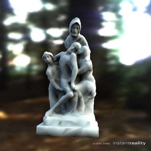
With all the knowledge we're now equipped with, we can build an X3D application using PRT. The following image is an example result with a low polygon model attached to this tutorial. The transfer coefficients for this model were computed with a diffuse shadowed transfer function, i.e. the transfer encodes diffuse reflection and soft self-shadowing. A SkydomeBackground has been added to include the spherical image in the background.
Rotating coefficients
When rotating an ordinary object, the normals are used after the rotation, as usual, to determine the lambert factor for each light source. If we think back however, the transfer function that was calculated at each vertex and moved to a set of coefficients has used a fixed normal. So an object whose color reflection is determined via PRT can be rotated, but the coefficient data and thus the lighting stays the same. The problem is obvious: whereas the object has been rotated in euclidian space, the frequency space counterpart that now saves all the reflection and BRDF data has not. There are three solutions to this problem.
The first and admittedly naive one is to recalculate all coefficients for each vertex with the newly rotated normal and position. This way we'll loose the realtime relighting benefit, so it is not an option.
The second method is to rotate the image or function we're using for the incident light in its own space in the opposite direction and then resample it to gain the coefficients. So for instance, we could devise an algorithm to rotate a latitude-longtitude map in pixel-space, use the rotation matrix of the object, invert it and apply this rotation to the image. The new coefficients can then be applied to the object. This method is way more efficient than the first one, but still not satisfying, as we have to keep track of the kind of parameter space of the incident light to rotate it the right way.
The third way is to use spherical harmonic rotation, which is a method to create a matrix that can rotate the coefficient vector. This type of matrix is called SphericalHarmonicsMatrix and can be defined as follows:
Code: A 16x16 (4x4 bands) spherical harmonic rotation matrix created from an ordinary 4x4 matrix.
<SphericalHarmonicsMatrix DEF='shMatrix' bands='4' rotation='
		1 0 0 0
		0 1 0 0
		0 0 1 0
		0 0 0 1'/>

ROUTE shGenerator.coefficients_changed TO shMatrix.set_coefficients
ROUTE shMatrix.coefficients_changed TO shShader.set_coefficients
And that's about it. Routing any matrix to the rotation field will create a new spherical harmonics matrix that in turn will transform an incoming coefficients vector to a rotated coefficients vector. By placing the inverse rotation matrix of the object into the SphericalHarmonicsMatrix times the rotation matrix of the surrounding Skydome, the object and the surrounding image can be rotated arbitrarly. The sample attached to this tutorial also includes rotation.
Files:
Comments
This tutorial has no comments.
Add a new comment
Due to excessive spamming we have disabled the comment functionality for tutorials. Please use our forum to post any questions.